Author: Krzysztof Satola (satola.net)
From: https://github.com/ksatola
Version: 1.0.0

Effectiveness of Different Analytical Techniques – Statistical and Machine Learning Models – in Particulate Matter Fine Particles Level Forecasting

About

According to the World Health Organization (WHO), air pollution is the biggest environmental risk to health in the European Union (EU) causing each year about 400 000 premature deaths, and hundreds of billions of euro in health-related external costs. The goal of this study is to describe efforts and scientific method for comparison effectiveness of different analytical techniques which can be used to predict fine particles of particulate matter (PM2.5) levels (as the most harmful pollutant). The insights and methods, like the best performing group of algorithms will be used in later iterations to build an interactive tool for PM2.5 level forecasting.


Table of Contents

  1. Problem Statement
  2. Research Goal, Approach and Outcome
  3. Technical Project Environment Setup
  4. Data Preparation
  5. Exploratory Data Analysis
  6. Modelling and Performance Comparison Method
  7. Hyper-parameters Tuning and Model Quality Evaluation
  8. Results
  9. Further Work
  10. Summary
  11. Resources

go up

Problem Statement

According to the World Health Organization (WHO), air pollution is the biggest environmental risk to health in the European Union (EU) causing each year about 400 000 premature deaths, and hundreds of billions of euro in health-related external costs [1]. Air pollution occurs when gases, dust particles and smoke are released into the atmosphere, making it harmful to humans, infrastructure and the environment. Particulate matter, nitrogen dioxide and ground level ozone are the air pollutants responsible for most of these early deaths.

We call smog any combination of air pollution, with or without humidity. The term smog (from smoke and fog) was created in early 1900s by the British researcher and doctor H.A. Des Voeux who conducted a research on after effects of air pollution problems in Glasgow and Edinburgh in autumn 1909, resulting in 1000 deaths [9].

The history of the problem of smelly smoke produced by forges, mines and other production facilities is very old. In 1273 the first known regulation was made in London regarding forbidden use of powdered coal. Since then there were many efforts put in place to control and improve air in big European and US cities. In 1775, Percival Pott, a well-known surgeon from London, described many cases of skin cancer of chimney sweeps and linked them to a contact with carbon black. In the industrial era, steam engines of steam locomotives, ships and factory machines became major pollution contributors. In 1888, a French professor Maximilien Ringelmann, invented the first way of pollution measurement, a few years later (1906) the first electrical precipitator was made. In the 20th century, new sources of pollution became apparent – cars and planes. The air pollution and associated with it global warming are considered one of the most serious civilizational and environmental challenges of the contemporary world [9].

There are two dimensions of air pollution and smog – global and local. Globally, it affects global warming. Locally, it influences quality of life and health of people living in different areas.

In Poland, environmental awareness started growing slowly in the mid-1950s, but mainly in academia. While the western world put a lot of effort into diversification of energy sources with the main goal of reducing coal, in Poland coal still remains the mainstay of energy source [2]. In the public debate, the main arguments against coal usage reduction are the need of mining industry preservation and destitute society not being able to afford modern, low emission solutions. While the world was improving, many Polish regions and cities started leading in pollution rankings. The quality of life – mainly during autumn and winter months – dropped drastically. Ultimately, in the 1990s consistent monitoring programs were put in place and various improvement programs were introduced (with the main contribution of UE regulations and funds) [4]. Unfortunately, the change happens very slowly, mainly due to people's awareness of the problem growing slowly and the limited knowledge of how the improvement should be handled efficiently.

The WHO identifies particulate matter (PM), nitrogen dioxide (NO2), sulphur dioxide (SO2) and ground-level ozone (O3) as the main air pollutants that are most harmful to human health. The most dangerous of them are fine particles (PM2.5) which caused about 400 000 premature deaths of EU citizens in 2014 (and similarly in every consecutive year) [1]. Smog cannot be contained by authorities or environmental services alone. It can be only tamed by everyone, including ordinary people who need to understand how bad the smog is and act to replace cacoethes of burning garbage and (low-calorie) coal resulting in harmful substances in the air. It can be tamed by industry, another significant source of smog. In order to reduce it, we need to increase usage of ecological methods of heating but also in energy (power stations) and industrial production. Replacing old furnaces with modern ones with use of air cleaners could also help.

Air quality does not only depend on pollution emissions. It also depends on proximity to the source and altitude at which pollutants are released; meteorological conditions, including wind and heat; chemical transformations (reactions to sunlight, pollutant interactions); geographical conditions (topography). Air pollution emissions result mostly from human action (as stated before) but they can also result from forest fires, volcanic eruptions and wind erosion. Air pollution is natural but its extend in the modern world is not [9].

Smog can be very sneaky. It may have greater impact on children who, when become adult, may suffer from diseases related to chemical compounds cumulated in their bodies. That is another reason why it is so important to eliminate smog (long-term) and avoid open air activities (short-term) when smog concentration outside is too high.

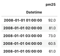
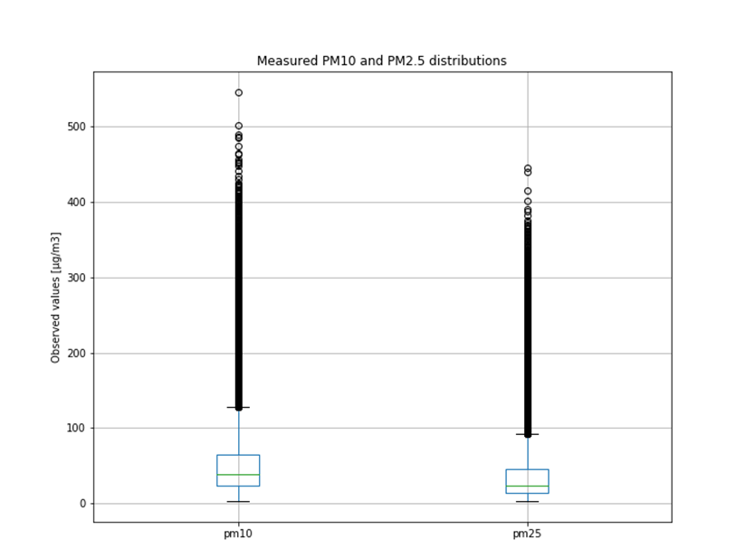
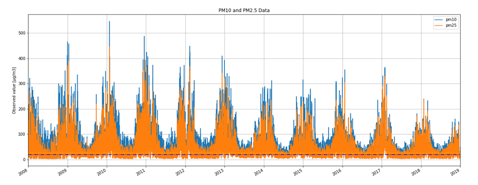
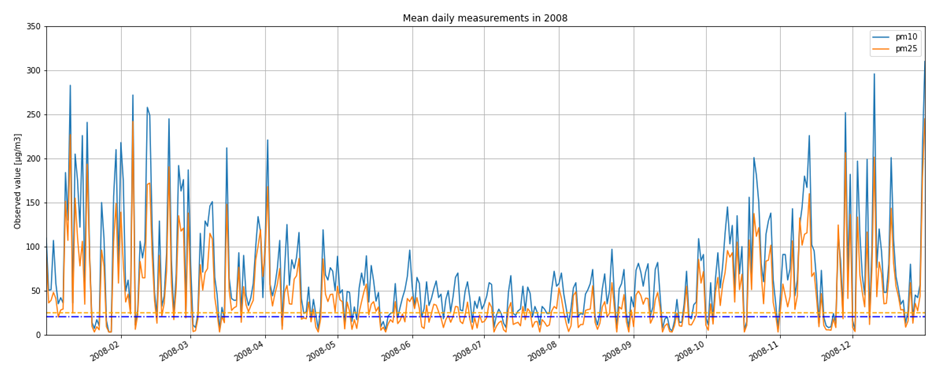
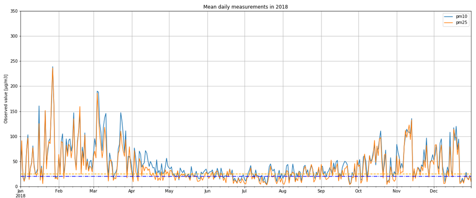
It is not only important to reduce air pollution but also to understand current air conditions around us to passively reduce its impact on our health by limiting our exposure. This is the main reason for the research described in this study – based on existing air pollution sensors' measurements (collected in the Kraków area, a high pollution hotspot). Kraków - my home city - struggles with very poor air quality, particularly during the winter season. Concentrations of particulate matter (PM10 and PM2.5) and benzo(a)pyrene are exceedingly high throughout the whole region.

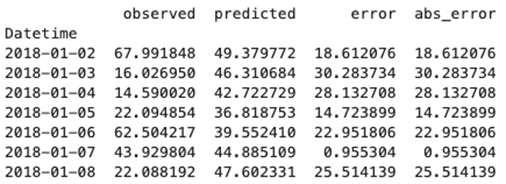
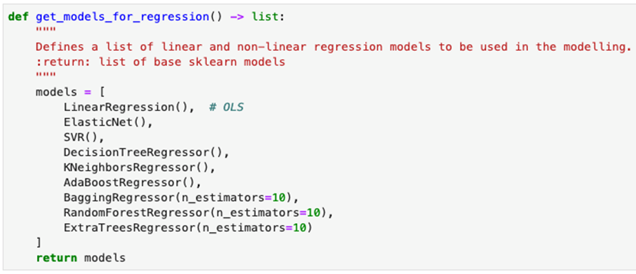
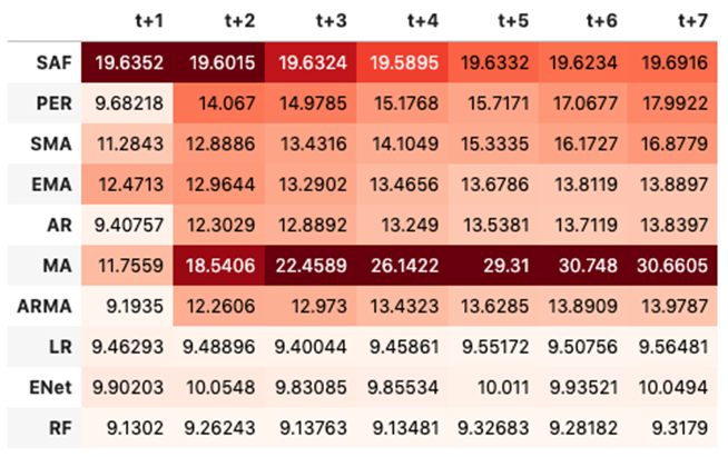
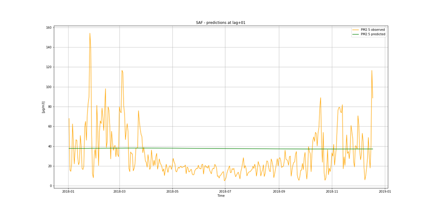
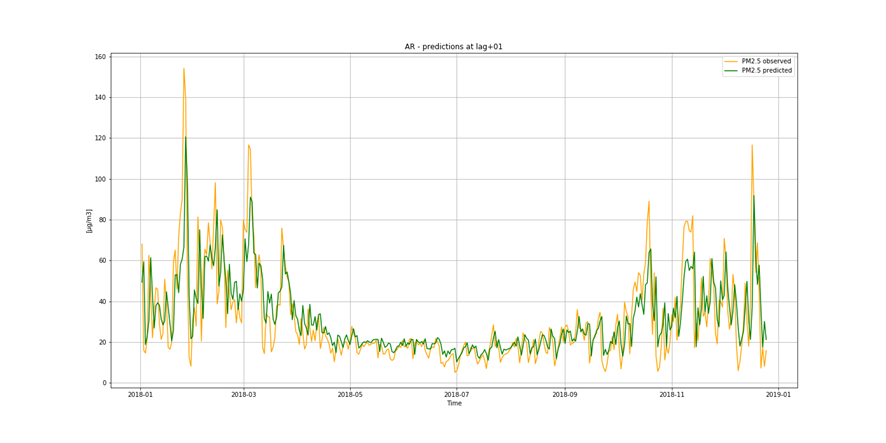
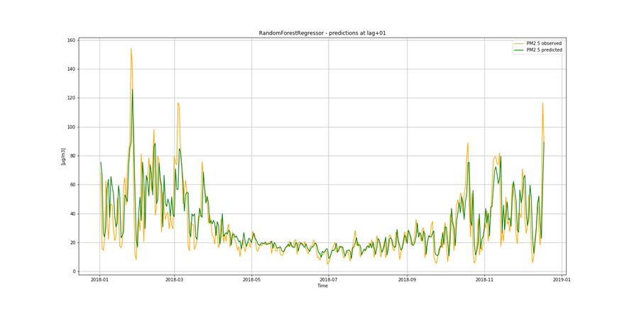
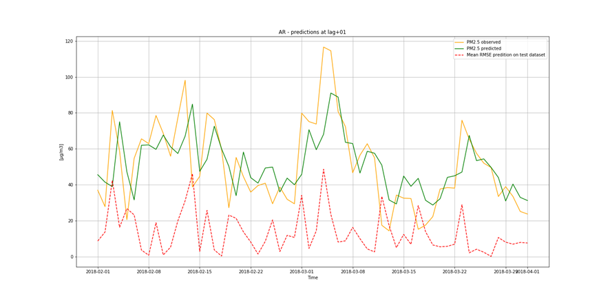
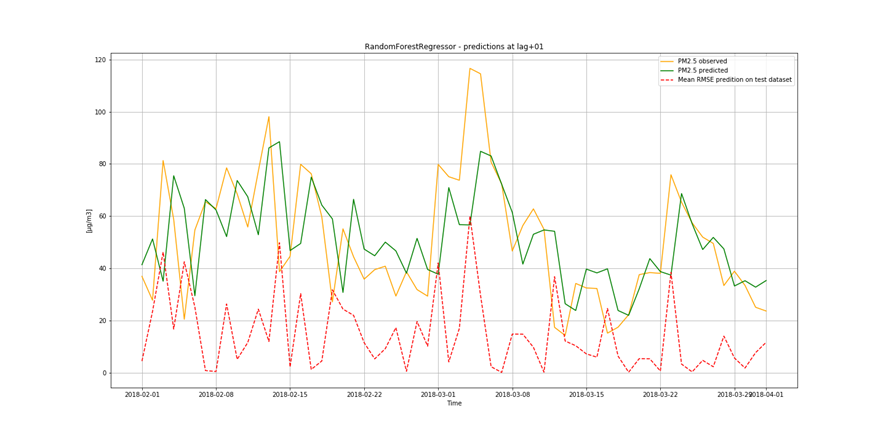
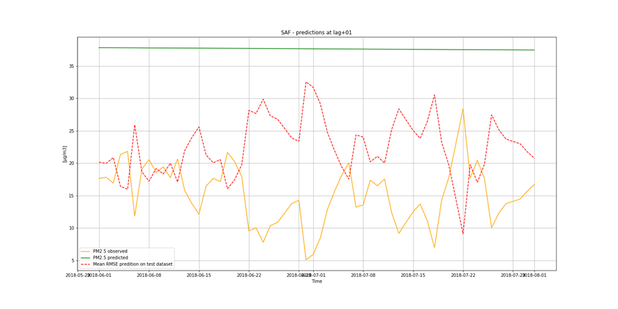
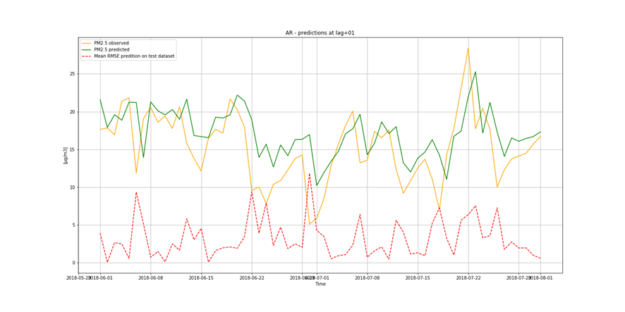
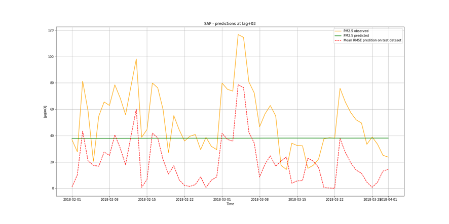
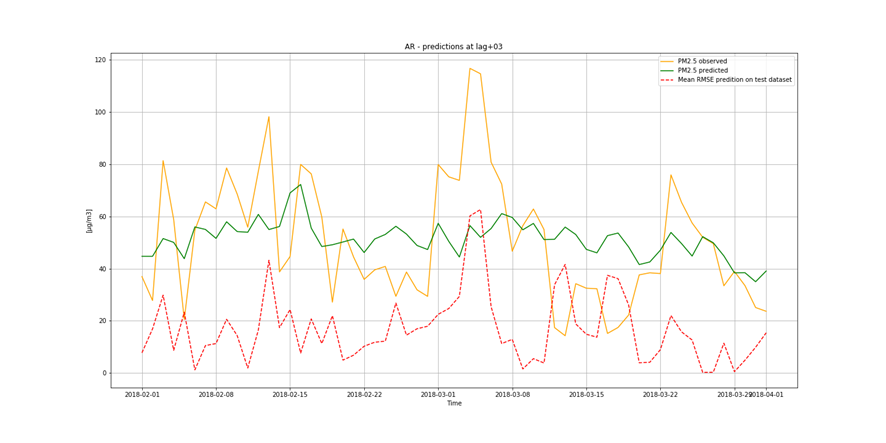
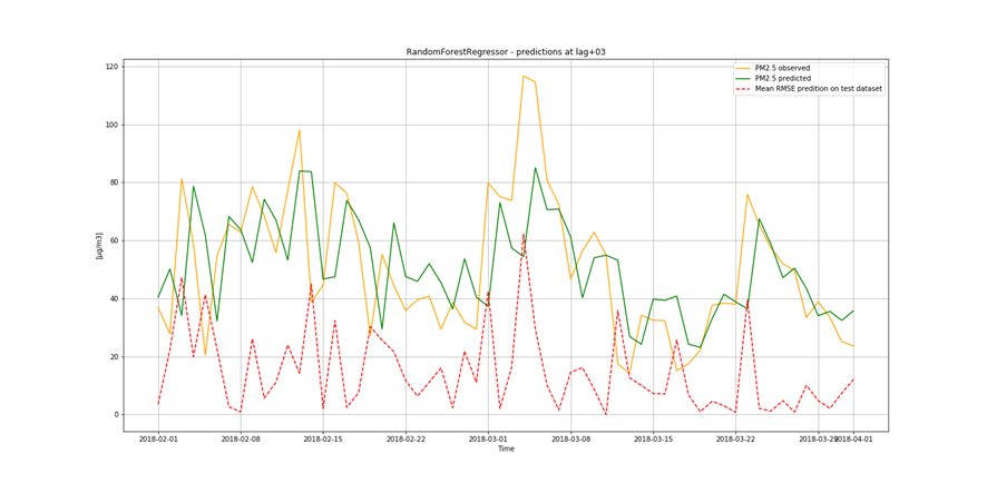
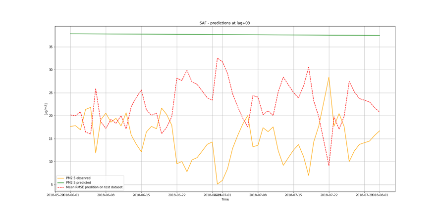
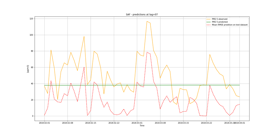
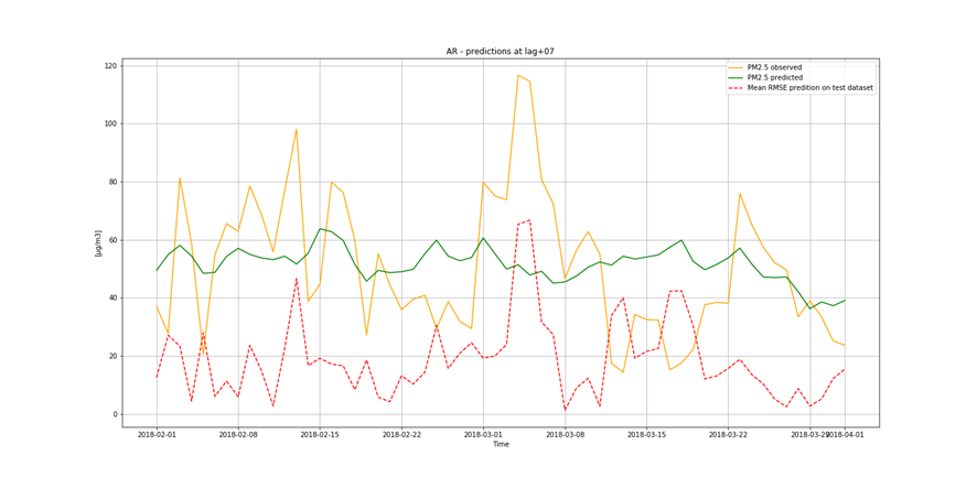
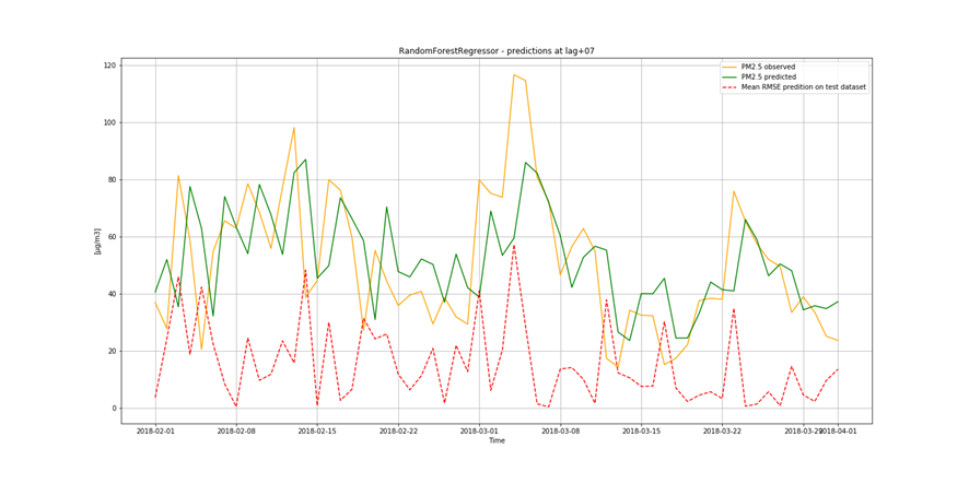
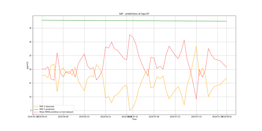
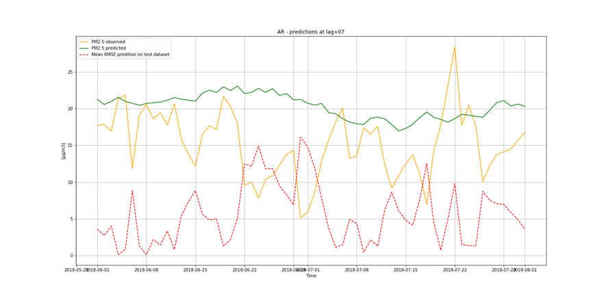
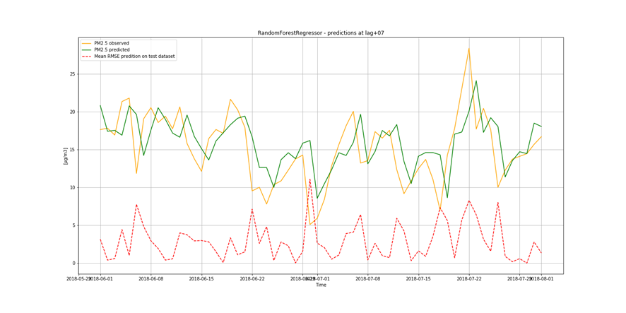
It is important to find best analytical methods for predicting fine particles of particulate matter (PM2.5) level. This could help ordinary people in planning any activities in the open air and reduce impact the air pollution makes to their health.


go up

Research Goal, Approach and Outcome

Research Goal

The goal of this dissertation is to describe efforts and scientific method for comparison effectiveness of different analytical techniques (basic, statistical and machine learning models) which can be used to predict fine particles of particulate matter (PM2.5) levels (time series univariate forecasting problem). The insights and methods, like the best performing group of algorithms will be used in later iterations to build a tool for PM2.5 level forecasting.

Approach (first iteration)

The problem solution can be divided into following phases (Scientific Method):

  1. Define the problem.
  2. Research the study area (both in terms of subject matter area (air pollution) and analytical methods).
  3. Define the goal, method and deliverables (study operationalization).
  4. Setup an analytical environment and best tools for the job.
  5. Collect and pre-process data.
  6. Explore and visualize data (statistical analysis).
  7. Evaluate and compare performance of different available analytical techniques for PM2.5 forecasting (univariate time series modelling).
  8. Implement a system (script and automate).
  9. Present results.
  10. Define next iteration steps.

Outcome

The outcome of this phase are:

All outcomes are stored and maintained for reproducible research in my Github repository.


go up

Technical Project Environment Setup

There are a few technical options for a data science project setup: Python, R, cloud analytical services (AWS SageMaker, Azure ML) or locally installed software like IBM SPSS or KNIME, to name a few. The approach and toolkit should be chosen based not only on the data scientist's personal preference and professional skills but mainly based on how it would fit the business problem solution’s requirements, cost and timing. How the data product is meant to be used and maintained after it is created and by whom. What the other factors are which could impact technical decisions. Last but not least, it is a good practice to strive for consistency which makes the learning curve for all project team members shallower, this is valid not only for a single project but also for a portfolio of all projects being executed in a company, institution or any other kind of organization, or by any group.

Python

This project’s technical components are based mainly on Python-related tools and modules. Mainly, because most of the analytical components needed are natively available in Python, but also because the final data product is a web app which should be easily customizable. Building all the pieces in Python, allows full flexibility and increases the speed of combining different components. It also makes it easier and faster to join ready-to-use components with custom code. Python virtual environment is used to separate the dependencies required by this project from all other ones and a global Python configuration on development machines.

Source Code Repository

To manage and share the project's code, Git and its free web version (github) is used. Git is a free and open source distributed version control system designed to handle everything from small to very large projects with speed and efficiency.

Jupyter Notebook

As a lab environment for experimentation and prototyping, Jupyter Notebook is used (or its more IDE-like version – Jupyter Lab). The Jupyter Lab is a web-based interactive development environment for Jupyter notebooks, code, and data. The Jupyter Notebook is an open-source web application that allows you to create and share documents that contain live code, equations, visualizations and narrative text. Uses include data cleaning and transformation, numerical simulation, statistical modeling, data visualization, machine learning, and much more.

Integrated Development Environment

As for quick experimentation and work documentation Jupyter is the right choice, nut for Python code long-term structuring and development, "The Python IDE for Professional Developers" – PyCharm is the tool of my choice (but other tools can be also as good as PyCharm is, or better). It is full-fledged integrated programming environment (IDE) with many configuration and extension options. It is a good choice for Python programming as it can be used for free (Community Edition) and supports good programming practices.

The detailed instructions are covered in the Project Environment notebook.


go up

Data Preparation

Extract Transform Load (ETL)

For this project, two main data sources are identified as the most comprehensive:

For both sources, different web scraping and data transformation techniques were used. The Extract Transform Load (ETL) process is fully automated, so the data can be updated easily in the future. The details (method description, code and results) can be found in the following notebooks:

In the first iteration of the project, only GIOS data is used (PM10 and PM2.5) as the main goal is to check which methods best apply to PM2.5 time series forecasting.

Datasets for Modelling

There are 2 types of datasets prepared for:

The data is adjusted for the following kinds of forecasts:

For this dissertation, selected algorithms were compared based on daily data, although the method and scripts work with hourly data as well. The reason for this is the additional time needed for calculations on the hourly dataset with more data points to forecast (the time difference between daily and hourly calculations is exponential, leading to hundreds of hours per model needed to perform certain calculations). This limitation will be overcome with more robust computational environment being prepared for next phases.

The datasets structure used for the basic and statistical methods is depicted in figure 5.1. The shapes of these datasets are (rows 96 388, column 1) for the hourly data, and (4 019, 1) for the daily data.

Figure 5.1. First five rows of the hourly dataset used for basic and statistical methods.

For the machine learning methods, instead of dealing with datetime index and time series values, there are additional features created based on time series lags and the time component taken from the datetime index of the original data structure (figure 5.2). The shapes of these datasets are (96378, 13) for the hourly data and (4015, 13) for the daily data. The difference in the rows number between the two types of datasets are a result of creating lagged columns (using the shift method creates columns with NaN (not a number) values which must be removed). The target column name is ‘t’.

Figure 5.2. First five rows of the daily dataset used for machine learning methods.

The number of lags were taken based on correlation coefficients (Pearson method) calculated between independent and dependent variables and is 4 for the daily dataset and 10 for the hourly one.

Features engineering is the process of transforming raw data into features that better represent the underlying problem to the predictive models, resulting in improved model accuracy on unseen data. For machine learning models, instead of dealing with datetime index, lag-based and datetime-based additional features were created and included in the analytical view. The lag-based features are described in the previous section. The datetime-based features were extracted from the datetime information associated with every time series value. The figure 5.3 shows the code snippet of build_datetime_features() function building datetime-based columns.

Figure 5.3. Datetime-based feature engineering method.

The details of analytical views preparation are covered in the Prepare Data for Modelling notebook.


go up

Exploratory Data Analysis

The Exploratory Data Analysis (EDA) covers particulate matter (PM) air pollutants with a special attention to fine particles (PM2.5) which are considered the most harmful out of all air-pollutants[1].

The dataset used in EDA contains hourly measurements of particulate matter (PM10) and fine particles (PM2.5) taken in Kraków area in the years of 2008-2018. There are 96 388 observations and no missing data.

The maximum values observed are 546 [µg/m3] for PM10 and 445 [µg/m3] for PM2.5, both on 2010-01-27 at 6am. The mean values are respectively 53 and 37 [µg/m3]. 75% of all observations are below 65 and 45 [µg/m3]. Almost 75% of PM10 and almost 50% of PM2.5 observations exceed WHO air quality guidelines (20 [µg/m3] for PM10 and 25 [µg/m3] for PM2.5) [2]. PM10 and PM2.5 distributions (figure 6.1) are similar (right-skewed) with many outliers at the high-end many times exceding WHO and EU air quality guidelines [2].

Figure 6.1. PM10 and PM2.5 distributions.

There is yearly seasonality in PM10 and PM2.5 data with the values increasing from October to April. PM10 and PM2.5 levels are similar, strongly and positively correlated (very strong Pearson's correlation coefficient: 0.96). This should not be surprising as PM2.5 is contained in PM10. The highest measurement values were taken between 2009 and 2011 (figure 6.2).

Figure 6.2. PM10 and PM2.5 data.

The characteristics of measurements look similar in all years (figure 6.3 shows the edge cases – 2008 and 2018 years). In autumn and winter, there are more air pollutants in the air then during the rest of the year. Looking at the vertical axes (the scale is standardized to be the same) we can clearly see, that situation is improving – the maximum values observed are lower in 2018 comparing to 2008 but are not still at the satisfactory level.

Figure 6.3. PM10 and PM2.5 data in 2008 and 2018.

Here are some other insights from the EDA:

Figure 6.4. PM10 and PM2.5 mean hourly distribution.

Figure 6.5. Weekly average particle matter levels of PM10 and PM2.5 in 2008-2018.

The details of EDA including additional plots are covered in the EDA for PM25 notebook.


go up

Modelling and the Performance Comparison Method

Modelling

Making predictions about the future is called extrapolation in the classical statistical handling of time series data. More modern fields focus on the topic and refer to it as time series forecasting. Forecasting involves taking models fit on historical data and using them to predict future observations.

Performance Comparison Method

In order to compare performance of different techniques which can be used for the time series forecasting, there must be developed a common testing approach (test harness). It must be the same to all methods (fair, comparable and representative to all data) and comprise of:

These common elements of the test harness are prepared in a central codebase. The model performance metric chosen for this exercise is: Root Mean Squared Error (RMSE), the most common and universal performance metric used for regression problems.

Base, statistical and machine learning models work differently, so the model fitting and predicting procedures are different for each kind of the method. In all cases models are trained on the train data and validated (tested) on non-seen data – the test dataset.

For the purpose of this exercise, a custom validation procedure (leveraging Walk-Forward Validation approach) on test data was developed. It is applied commonly to all models and works as follows:

  1. Take a test dataset as a truth about quality of prediction of different methods. As there is yearly seasonality and you want to be fair while comparing different models, use entire year as test data, so it represents all possible kinds of cases for prediction. This is important, as some of the models show different level of performance depending on the history-future split point in time.
  2. Divide the test data into folds. Folds start at each data point of the test set (daily for the daily data and hourly for the hourly data) and contain as many values as required for long-term prediction (7 for the daily data and 24 for the hourly data).
  3. For each fold:
    1. Forecast values one by one, starting from lag+1 to lag+7 or lag+24, replacing the historical data (shifted one by one into the future) with just made predictions. The further in the future, the bigger error is expected to be generated by this forecasting method.
    2. Gather results (figure 7.1), calculate RMSE of the fold's forecasts and observed values (from the test dataset).
  4. Average RMSEs per each lag+n forecasted values across all folds.
  5. Compare performance of the different methods numerically and graphically.

Figure 7.1. Exemplary result for a 7-day fold.

Figure 7.2 shows a simplified snapshot of a validation procedure code. The procedure is planned to be refactored (during the next iteration, based on learnings from the current phase of the project) and code structure for different methods standardized. The method specific details and differences will be read from external JSON configuration files, but the current validation logic will remain intact.

Figure 7.2. Snapshot of a validation procedure code for ARMA method.

Baseline Reference Methods

Establishing a baseline is essential on any time series forecasting problem. A baseline on forecast performance provides a point of comparison. It is a point of reference for all other modeling techniques. If a model achieves performance at or below the baseline, the technique should be fixed or abandoned.

The technique used to generate a forecast to calculate the baseline performance must be easy to implement and naive of problem-specific details. Three properties of a good technique for making a baseline forecast are:

Techniques

The base techniques selected for the comparison are:

The chosen models are simple, fast and deterministic. The implementation and validation details are documented in the Baseline Reference Models notebook.

Statistical Methods

Assumptions

A time series is a data sequence ordered (or indexed) by time. It is discrete, and the interval between each point is constant. This dissertation focuses on univariate time series forecasting with different methods. Univariate time series are datasets where only a single variable is observed at each time (PM2.5).

Statistical methods often have assumptions which should be checked before a method is applied. The main assumptions for time series forecasting using statistical methods are:

The first assumption is: The previous time step(s) – lag(s) – is useful in predicting the value at the next time step (dependence between values). If the time series data values are independent of each other, autoregressive model isn’t going to be a good forecasting method for that series (no correlation). This assumption can be checked by looking at the plot of entire time series (figure 7.3) and calculating autocorrelation between the time series and its lags (figure 7.4).

Figure 7.3. Correlogram plot of entire PM2.5 time series.

Figure 7.4. Pearson correlation coefficients for PM2.5 time series and its t-n lags.

What we can see yearly seasonal cycles (figure 7.3) and the most influencing (autocorrelated) daily lags being closer to the observation point at lag 0 (figure 7.4). The first lagged value is highly correlated to the times series (correlation coefficient higher than 0.7), and this correlation is statistically significant. For the dataset for statistical methods modelling 3 more lags are considered for the modelling (t-2, t-3 and t-4). All of them are statistically significant, too. After lag 4, we observe steady decline of correlation coefficient value.

The second assumption is: The time series data is stationary. The time series is stationary if its mean (and/or variance) is constant over time (over a specified time range). If the time series data isn’t stationary, it should be made that way with some form of trend and seasonality removal (decomposition) or an application of so-called power transform. In order to check for stationarity, 2 tests were performed on PM2.5 data:

Figure 7.5. PM2.5 data variability of mean and variance.

The variability check was made by dividing entire time series into unequal folds, calculating mean and variance for each fold separately and comparing them to find if there were significant differences. Based on figure 7.5, we may conclude, that the PM2.5 data is stationary.

Figure 7.6. The Augmented Dickey-Fuller unit root test in results.

The Augmented Dickey-Fuller unit root test calculates a test statistic, which in PM2.5 case equals to minus 5.37. This number is lower than any of the critical values, so we can conclude with 99% of certainty, that PM2.5 time series is stationary.

As a result of PM2.5 time series diagnostics, we can say that PM2.5 data is stationary and there is no need for detrending nor application of any of power transformations. The previous time step(s) can be used in predicting the value at the next time step. As PM2.5 data is stationary, checking statistical models makes sense. For statistical modeling PM2.5 data can be used as-is.

Other details of the diagnostics phase can be found in the Time Series Decomposition and Time Series Correlations notebooks.

Techniques

The statistical techniques selected for the comparison are:

Machine Learning Methods

Best Models Selection

There are hundreds of Machine Learning (ML) methods to choose from. For the purpose of this comparison there is a selection method proposed and evaluated in the following way:

  1. Start with an arbitrary but representing different types selection of linear and non-linear regression models available in scikit-learn Python library (figure 7.7).
  2. Fit the models on the train dataset and calculate RMSE on the train dataset. For the fitting use k-fold cross-validation method to reduce over-fitting (figure 7.8).
  3. Rank the models based on their RMSE (figure 7.9) and choose 3 best performing models (linear and non-linear).
  4. Perform grid-search or randomized search to find potential better hyper-parameters than default ones (see the next section for details).
  5. Evaluate the best models using grid-search or randomized search results and the common model performance comparison method.

Figure 7.7. Regression estimators in scope.

Figure 7.8. Machine learning models ranking method.

Figure 7.9. Ranking of machine learning models.

The best performing algorithms are LinearRegression (RMSE on train 21.71) and ElasticNet (RMSE on train 21.83). They are both linear estimators. The best non-linear estimator is RandomForestRegressor (RMSE on train 23.21). As it is good to have a wide representation of techniques for the comparison, these three ML models were fine-tuned and compared with other time series forecasting techniques.

Techniques

According to the initial ranking, the best machine learning models to forecast PM2.5 are:

More details regarding PM2.5 machine learning modelling can be found in the Machine Learning Regression notebook.


go up

Hyper-parameters Tuning and Model Quality Evaluation

During this research, different methods were used to find optimal hyper-parameters for different models:

AR Model

Statsmodels’ function AR() used for AR modelling, provides suggestions regarding number of lags which should be used by the estimator. In the case of PM2.5, the function suggested 30 lags to be used. The quality check on the fitted model residuals showed no more statistically significant lags left (figure 8.1), so AR(30) was used in the modelling.

Figure 8.1. AR fitted model residuals autocorrelation and partial autocorrelation plots.

MA, ARMA, ARIMA Models

For MA, ARMA and ARIMA models the best set of parameters for PM2.5 modelling was estimated by using the common procedure (figure 8.2).

The get_best_arima_params_for_time_series() function builds a list of possible combinations for ARIMA p, d, q maximal parameters (because of computational limitations, the maximum values for the parameters, were respectively 5, 2 and 5). Then, for every combination, the Akaike Information Criterion (AIC) estimator of out-of-sample prediction error (relative quality of statistical models for a given set of data) was used. Given a collection of models for the data, using AIC metric the best model was selected (figure 8.3).

For this particular example (figure 8.3) it is interesting to notice, that the best set of parameters for ARIMA (for the hourly data) does not include the differencing parameter (d=0). ARIMA(5, 0, 3) selected by AIC in this case is the same as ARMA(5, 3). This can even more strongly suggest, that PM2.5 (hourly) time series is stationary. Another thing worth noticing is the wall time of 49 minutes for hourly data, comparing to 3 minutes needed for the same estimation for daily data.

Figure 8.2. Estimation of best parameters for MA, ARMA and ARIMA models.

Figure 8.3. AIC results comparison for ARIMA model (hourly data).

In terms of quality of models, for each of the statistical models, a fitted model predicted coefficients (on train dataset) were compared to observed ones. For the t+1 prediction, all models performed very well. Figure 8.4 shows the comparison for MA(5) model. It is worth noticing, that all ma coefficients are statistically significant (P>|z| column is less than 0.05).

Figure 8.4. The comparison of predicted vs. observed coefficients for MA(5) model.

For each of the statistical models the fitted model residuals (errors) were evaluated. In short, the better the model, the less residuals are statistically significant, the distribution of the residuals is closer to normal, and the standardized residuals are white noise (not predictable random signal). Figure 8.5 shows fitted ARMA(5, 0, 4) model quality diagnostics. It does not look bad, nevertheless the Q-Q plot could fit better the red line.

Figure 8.5. Fitted ARMA(5, 0, 4) model quality diagnostics.

Machine Learning Models

The three best performing regression estimators: LinearRegression, ElasticNet and RandomForestRegressor were subject to hyper-parameters tuning procedure. Hyper-parameters are parameters that are not directly learnt within estimators. In general, there are two most used methods of ML hyper-parameters tuning: GridSearchCV (figure 8.6) and RandomizedSearchCV. The first method exhaustively considers all parameter combinations for given values. The second can sample a given number of candidates from a parameter space with a specified distribution. It is common that a small subset of those parameters can have a large impact on the predictive or computational performance of the model while others can be left to their default values.

Using RandomizedSearchCV has two main benefits over an exhaustive search:

For the purpose of PM2.5 time series forecasting, both methods were used. The first one on LinearRegression and ElasticNet, and the second on RandomForestRegressor.

Figure 8.6. GridSearchCV function.

While searching for best hyper-parameters, a technique called Cross-Validation (CV) is used to address a risk of model over-fitting. This technique prevents test data set leaking into training process. In CV, the training data is divided to folds and one of the fold acts as a validation dataset and the test dataset is still held out for final evaluation [13]. This approach is used for PM2.5 forecasting regarding all training and testing activities regardless of the model type (but the implementations differ).


go up

Results

The compared models are summarized in the table 9.1.

Table 9.1. Models in scope of the comparison.

Table 9.2 depicts the comparison of performance results for all models of all types. It shows models’ absolute (different scales per model) performance (forecasting t+n prediction point). This summary is done for the daily data (up to 7-days prediction). The performance metric, the goodness of fit, is the mean of Root Mean Squared Error (mean RMSE) – the smaller value, the better.

Table 9.2. Models’ absolute performance for t+n prediction points.

Most of the models predict better for smaller n. The greater n is, the greater error becomes. This is not the case regarding ML models, although the differences between t+n predictions are very small (usually around 9.5-10 [µg/m3]). The model that performs equally bad for all n is SAF. It was not too difficult to other models to outperform it.

Table 9.3 shows the comparison of performance results for all models of all types but this time in relation to other models. This summary is also done for the daily data (up to 7-days prediction). The performance metric, the goodness of fit, is represented by is the mean of Root Mean Squared Error (mean RMSE) – the smaller value, the better.

Table 9.3. Models relative performance for t+n prediction points.

Below, there is a comparison of predicted vs. observed values for t+1 (figure 9.4A, B, C), t+3 (figure 9.5A, B, C) and t+7 (figure 9.6A, B, C) forecasts for selected 3 models, each from a different group: SAF, AR and RF. The index by the figure number represents:

The most important observations which can be made from figures 9.4-9.6 are:

Based on numerical values and plots (tables and figures 9.2-9.6) we may conclude that the best performing group of models is machine learning. The RF model seems to be the best, although it did not show its strength so clearly during initial ML models rankings (most likely because of less sophisticated method of models’ comparison when it was ranked on the train dataset).

The worst models for PM2.5 time series are MA and SAF, this is due to PM2.5 time series distribution characteristics (part of time series high above its mean and another part all below the mean). The worst group of models are base models and statistical models can be placed in the middle in terms of their performance. It is worth noticing, that ML models’ performance is similarly independent of the n value (their RMSE level seems quite stable while n changes). For the most other models, n and RMSE are positively correlated, the greater n, the greater RMSE value.

Having said that, the RMSE still seems to be too high anyway, and existing models should be further fine-tuned, or new ones should be evaluated. As RF seems to provide the best results, other ensemble models should be tested as well.


Figure 9.4A. Comparison of predicted vs. observed values for t+1, for SAF, AR and RF (2018).


Figure 9.4B. Comparison of predicted vs. observed values for t+1, for SAF, AR and RF (February-March 2018).


Figure 9.4C. Comparison of predicted vs. observed values for t+1, for SAF, AR and RF (June-July 2018).


Figure 9.5A. Comparison of predicted vs. observed values for t+3, for SAF, AR and RF (2018).


Figure 9.5B. Comparison of predicted vs. observed values for t+3, for SAF, AR and RF (February-March 2018).


Figure 9.5C. Comparison of predicted vs. observed values for t+3, for SAF, AR and RF (June-July 2018).


Figure 9.6A. Comparison of predicted vs. observed values for t+7, for SAF, AR and RF (2018).


Figure 9.6B. Comparison of predicted vs. observed values for t+7, for SAF, AR and RF (February-March 2018).


Figure 9.6C. Comparison of predicted vs. observed values for t+7, for SAF, AR and RF (June-July 2018).


go up

Further Work

This dissertation reflects the status of the first iteration of the air-pollution forecasting project. There are multiple ways of continuing, but the following paths should be explored at the first place:


go up

Summary

The goal of this dissertation was to describe efforts and scientific method for comparison effectiveness of different analytical techniques which could be used to predict fine particles of particulate matter (PM2.5) levels (time series univariate forecasting problem).

In order to achieve the goal, air-pollution and climate data were scrapped from IMGW and GIOS web sites to create an analytical view (with only PM2.5 timeseries being in scope). Based on the view, an exploratory data analysis was performed, and then additional data transformation for modelling were made, with different resampling and feature engineering techniques. Different statistical methods were used to assess time series readiness for modelling (correlation and stationarity tests).

Three types of analytical techniques (basic, statistical and machine learning models) were used to create a ranking of best performing algorithms for PM2.5 forecasting. The method of comparison was mean RMSE and a custom validation function for fairness of results was created using walk-forward validation approach. Using the common validation approach the winner technique (Random Forrest regressor) and the best group (machine learning) were identified.

At the end, a proposal for further work was made with the main aim of improving forecasting and computational performance.


go up

Resources

  1. Air pollution: Our health still insufficiently protected (https://op.europa.eu/webpub/eca/special-reports/air-quality-23-2018/en/)
  2. European Environment Agency (EEA): Air Pollution (https://www.eea.europa.eu/themes/air)
  3. The European environment – state and outlook 2020 (http://www.gios.gov.pl/en/eea/highlights-eea-nfp-pl/649-the-european-environment-state-and-outlook-2020)
  4. LIFE Integrated Project "Implementation of Air Quality Plan for Małopolska Region – Małopolska in a healthy atmosphere" (https://powietrze.malopolska.pl/en/life-project/)
  5. Review of evidence on health aspects of air pollution – REVIHAAP Project, Technical Report (http://www.euro.who.int/__data/assets/pdf_file/0004/193108/REVIHAAP-Final-technical-report-final-version.pdf?ua=1)
  6. Zanieczyszczenie powietrza (Kraków) (https://powietrze.malopolska.pl/baza/jakosc-powietrza-w-polsce-na-tle-unii-europejskiej/)
  7. Time Series Forecasting: Principles and Practice (https://otexts.com/fpp2/)
  8. Forecasting Time Series Data using Autoregression (https://pythondata.com/forecasting-time-series-autoregression/)
  9. Smog w Polsce – przyczyny, skutki, przeciwdziałanie, Piotr Kleczkowski (PWN, 2020)
  10. Polish Institute of Meteorology and Water Management - National Research Institute (http://site.imgw.datatask.net/sites/default/files/IMGW_About_2019.pdf)
  11. IMGW data archive (https://dane.imgw.pl/data/dane_pomiarowo_obserwacyjne/dane_meteorologiczne/terminowe/synop/)
  12. Polish Inspectorate of Environmental Protection (http://powietrze.gios.gov.pl/pjp/archives)
  13. Cross-validation (https://scikit-learn.org/stable/modules/cross_validation.html)